Laplace Equation#
강좌: 기초 전산유체역학
Laplace Equation#
Laplace Equation은 비압축성, 비회전류 유동에서 정상상태일 때 Velocity Potential 또는 Streamfunction의 해이다.
간단한 예제로 Heat Conduction에 의해 Steady State에 도달하는 경우를 생각하자
예를 들면, 윗면에 온도만 300도이고 나머지 면의 온도가 100도인 경우 최종적으로 2차원 공간 내 온도 분포는 Laplace Equation으로 구할 수 있다.
\([0,1]^2\) 공간에 대해 수식으로 표현하면 다음과 같다.
편의상 \(k=1\) 로 생각한다.
Finite Difference Method#
그림과 같이 계산 영역을 x, y 각 방향별로 균일하게 나누어서 생각하자.
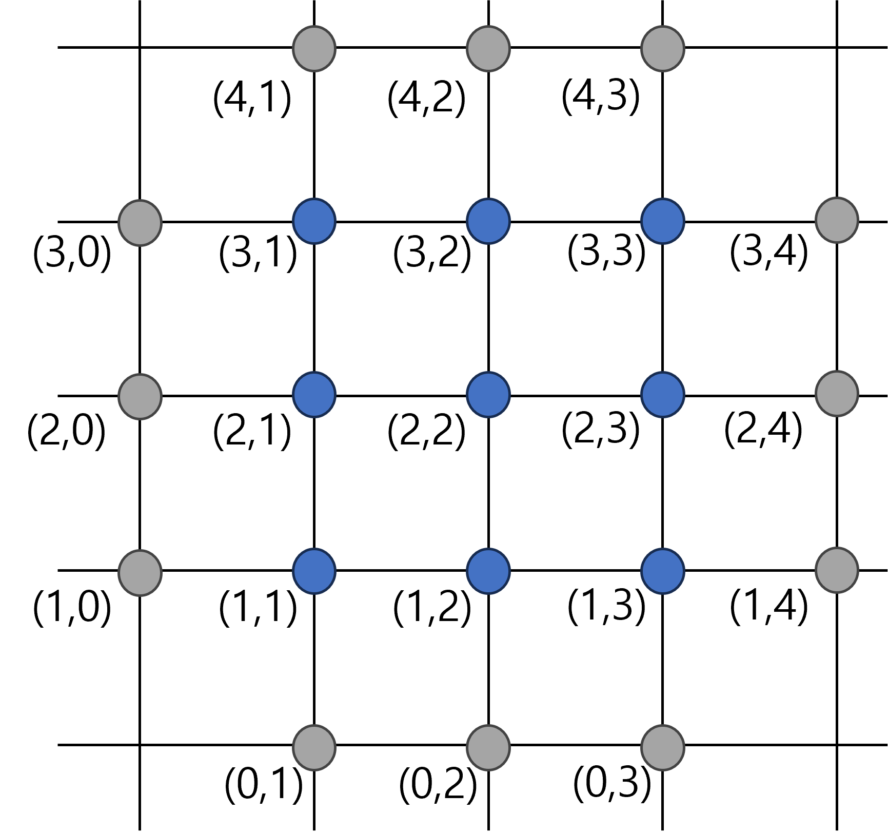
Fig. 13 Grid#
이 경우 2차원 Array는 각 격자점의 해와 부합한다.
각 방향별 편미분을 2차 정확도 Central Difference로 표현하면 다음과 같다.
\(\Delta x = \Delta y = h\) 인 경우 다음과 같이 정리된다.
이를 Matrix 형태로 나타내면 다음과 같다.
단 한번에 역행렬을 구함으로 써 모든 점에서 온도를 구할 수 있다.
다만 공간 차분 점이 늘어날수록 역행렬을 계산하는 시간이 급격하게 늘어난다.
예제#
Laplace 행렬을 구성한 후 Linear System을 해석하시오.
%matplotlib inline
from matplotlib import pyplot as plt

import numpy as np

plt.style.use('ggplot')
plt.rcParams['figure.dpi'] = 150
def laplace_op(n):
    """
    Laplace operator

    Parameters
    ----------
    n : integer
        size of system

    Returns
    -------
    a : matrix
        operator
    """
    a = np.zeros((n*n,n*n))

    for i in range(n):
        for j in range(n):
            if i == j:
                for l in range(n):
                    for k in range(n):
                        ii = n*i + l
                        jj = n*j + k

                        if l == k:
                            a[ii, jj] = -4
                        elif abs(l-k) == 1:
                            a[ii, jj] = 1
            elif abs(i-j) == 1:
                for l in range(n):
                    for k in range(n):
                        ii = n*i + l
                        jj = n*j + k

                        if l == k:
                            a[ii, jj] = 1
    return a
def bc(n):
    """
    Solution array with BC
    """
    x = np.zeros(n*n)

    for i in range(n):
        for j in range(n):
            if i == n-1:
                # Top
                x[n*i + j] -= 300
            elif i == 0:
                # Bottom
                x[n*i + j] -= 100
            if j == n-1:
                # Right
                x[n*i + j] -= 100
            elif j == 0:
                # Left
                x[n*i + j] -= 100

    return x
# Construct operator
n = 19
a = laplace_op(n)
x = bc(n)
# Solve
from scipy import linalg

tt = np.linalg.solve(a, x)
# Generate points (excluding BC)
xi = np.linspace(0, 1, n+2)
xx, yy = np.meshgrid(xi[1:-1], xi[1:-1])
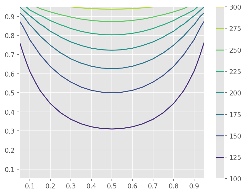
# Plot contour
plt.contour(xx, yy, tt.reshape(n,n))
plt.colorbar()
<matplotlib.colorbar.Colorbar at 0x7f219bb16d10>
Computational Costs#
선형 방정식의 계산은 Matrix-Matrix 곱 연산이다.
Matrix 곱 연산의 계산 시간은 \(O(n^3)\) 임
Matrix 곱셈 연산 속도 측정#
A (\(m \times n\)), B (\(n \times l\)) 곱셈 연산을 수행할 경우
A 행렬의 row vector와 B 행렬의 column vector 가 내적한다
\(a_1*b_1 + a_2*b_2\) : 2번의 곱셈 + 1번의 덧셈
\(2n-1 \approx 2n\) 번의 연산 (덧셈 & 곱셈)
m 개의 Row 와 l 개의 column 에 대해 연산을 반복한다.
총 \(2 m \times l\times n\) 번의 연산 수행
\(2 m \times l\times n\) Floating Points OPerations (FLOP)
GEMM (General Matrix to Matrix Multiplication)
대표적인 연산 속도 측정 방법
FLOPS : Floating Points OPerations per Second
%timeit함수를 이용해서 \(m=n=l=4096\) 인 경우 평균 연산 시간과 FLOPS를 측정하라사용중인 CPU의 이론 성능과 비교해보자
m=n=l=1024

a = np.random.rand(m, n)
b = np.random.rand(n, l)
c = np.random.rand(m, l)

t = %timeit -o c[:] = a @ b

flops = 2*m*n*l / t.average
print("Measured FLOPS : {:.4f} GFLOPS".format(flops*1e-9))
실습#
위 Laplace 방정식의 격자 개수를 늘려보자. 해의 변화를 관찰하고, 계산시간의 증가를 파악하라.
실습 페이지의 Poisson 방정식을 해석해보자.
Iterative Methods#
개념#
매우 큰 행렬 System \(Ax=b\) 를 반복해서 푸는 방법이다.
기본 개념은 다음과 같다.
\(A = A_1 - A_2\)
\(A_1\) 은 역행렬을 쉽게 구해지는 형태이다.
반복되는 해를 \(x^{(k)}\) 하고 이를 적용한다.
\(x^{(k)} \rightarrow x\) 이면 오차 \(e^{(k)} = x^{(k+1)} - x^{(k)} \rightarrow 0\) 이다. 즉 오차가 \(e^{(k)}\) 감소할 때 까지 반복한다.
모든 경우에 오차가 감소하지 않는다. \(A_1^{-1} A_2\) 의 Eigenvalue가 모두 1 보다 작아야 한다.
Point Jacobi Method#
이 방법은 \(A_1 = D\) 로 한 경우이다.
Laplace 문제에 적용하면 다음과 같이 표현할 수 있다.
def jacobi(n, ti, dt):
    """
    Jacobi method

    Parameters
    ----------
    n : integer
        size
    ti : float
        current time
    dt : array
        difference
    """
    for i in range(1, n+1):
        for j in range(1, n+1):
            dt[i, j] = 0.25*(ti[i-1, j] + ti[i, j-1] + ti[i+1, j] + ti[i, j+1]) - ti[i, j]

def jacobi_v1(ti, dt):
    """
    Jacobi method (Vector version)

    Parameters
    ----------
    n : integer
        size
    ti : float
        current time

    Parameters
    -----------
    dt : array
        difference
    """
    dt[1:-1, 1:-1] = 0.25*(ti[:-2, 1:-1] + ti[1:-1, :-2] + ti[2:, 1:-1] + ti[1:-1, 2:]) - ti[1:-1, 1:-1]
n = 19
tol = 1e-5
ti = np.zeros((n+2, n+2))
dt = np.zeros((n+2, n+2))

def bc(t):
    t[-1, 1:-1] = 300
    t[0, 1:-1] = 100
    t[1:-1, -1] = 100
    t[1:-1, 0] = 100

err = 1
hist_jacobi = []
while err > tol:
    # Apply BC
    bc(ti)

    # Run Jacobi
    jacobi(n, ti, dt)
    #jacobi_v1(ti, dt)

    # Compute Error
    err = linalg.norm(dt) / n
    hist_jacobi.append(err)

    # Update solution
    ti += dt
# Generate points (excluding BC)
xi = np.linspace(0, 1, n+2)
xx, yy = np.meshgrid(xi[1:-1], xi[1:-1])
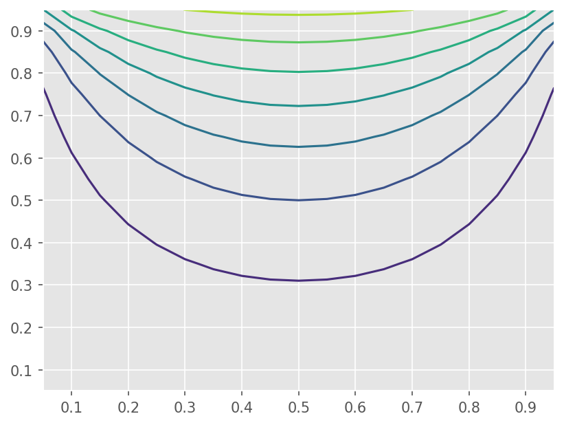
# Plot contour
plt.contour(xx, yy, ti[1:-1, 1:-1])
<matplotlib.contour.QuadContourSet at 0x7f219bb8fd50>
Gauss-Seidel#
\(A=L+D+U\) 라 생각했을 때 \(A_1 = L + D\)인 방법이다.
Laplace 방정식에 적용하면 다음과 같다.
def gauss_seidel(n, ti, dt):
    """
    Gauss-Seidel method

    Parameters
    ----------
    n : integer
        size
    ti : float
        current time
    dt : array
        difference
    """
    for i in range(1, n+1):
        for j in range(1, n+1):
            tij = ti[i, j]
            ti[i, j] = 0.25*(ti[i-1, j] + ti[i, j-1] + ti[i+1, j] + ti[i, j+1])
            dt[i, j] = ti[i, j] - tij
n = 19
tol = 1e-5
ti = np.zeros((n+2, n+2))
dt = np.zeros((n+2, n+2))

def bc(t):
    t[-1, 1:-1] = 300
    t[0, 1:-1] = 100
    t[1:-1, -1] = 100
    t[1:-1, 0] = 100

err = 1
hist_gs = []
while err > tol:
    # Apply BC
    bc(ti)

    # Run Gauss-Seidel
    gauss_seidel(n, ti, dt)

    # Compute Error
    err = linalg.norm(dt) / n
    hist_gs.append(err)
# Generate points (excluding BC)
xi = np.linspace(0, 1, n+2)
xx, yy = np.meshgrid(xi[1:-1], xi[1:-1])

# Plot contour
plt.contour(xx, yy, ti[1:-1, 1:-1])
<matplotlib.contour.QuadContourSet at 0x7f219803c910>

# Compute History
plt.semilogy(range(len(hist_jacobi)), hist_jacobi)
plt.semilogy(range(len(hist_gs)), hist_gs)
plt.xlabel('Iterations')
plt.ylabel('Error')
plt.legend(['Jacobi', 'Gauss-Seidel'])
<matplotlib.legend.Legend at 0x7f2198109710>
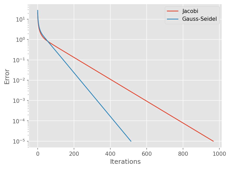
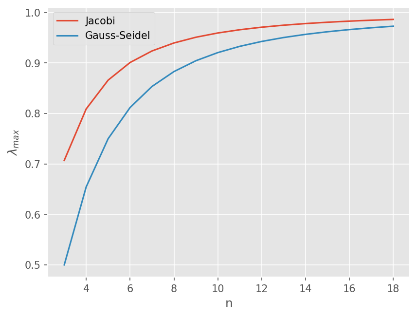
수렴 특성 비교#
오차 벡터 \(E^n\) 이라 할 때, 오차는 다음과 같이 감쇄한다.
\(E^{n+1} = (A_1^{-1} A2) E^{n}\)
즉 행렬 \(A_1^{-1} A_2\) 의 최대 Eigenvalue에 따라 오차 감쇄율이 달라진다.
행렬 크기를 3~19까지 최대 Eigenvalue 구하기
np.diag: 대각 행렬 항 구함, 주어진 대각 행렬로 구성된 행렬 구함np.tril: Lower triangle 행렬 계산linalg.inv: 역행렬 계산linalg.eig: 행렬의 Eigenvalue와 Eigenvector 계산
# 행렬의 크기
ns = range(3, 19)

# Jacobi 방법의 최대 고유치 계산
ev_jacobi = []

for n in ns:
    A = laplace_op(n)

    # Jacobi 방법을 행렬로 표기
    A1 = np.diag(np.diag(A))
    A2 = A - A1
    op = linalg.inv(A1) @ A2

    # 최대 고유치 계산
    evi = np.abs(linalg.eig(op)[0]).max()
    ev_jacobi.append(evi)

ev_gs = []

for n in ns:
    A = laplace_op(n)

    # Gauss-Seidel 방법을 행렬로 표기
    A1 = np.tril(A)
    A2 = A - A1
    op = linalg.inv(A1) @ A2

    # 최대 고유치 계산
    evi = np.abs(linalg.eig(op)[0]).max()
    ev_gs.append(evi)

plt.plot(ns, ev_jacobi)
plt.plot(ns, ev_gs)
plt.legend(['Jacobi', 'Gauss-Seidel'])
plt.xlabel('n')
plt.ylabel(r"$\lambda_{max}$")
Text(0, 0.5, '$\\lambda_{max}$')
Succesive overelaxation (SOR)#
Gauss-Seidel 결과에 relxation parameter \(\omega\) 를 이용해서 계산 결과를 가속한다.
즉
여기서 \(\tilde{T}_{i,j}^{(n+1)}\) 은 Gauss-Seidel 결과이다.
실습#
SOR 방법을 구현하시오. \(\omega \in (1.1, 1.8)\) 사이에서 값을 변화시키면서 수렴 속도를 비교하시오.
Point Jacobi, Gauss Seidel, SOR 방법에 대해 격자 크기를 달리하면서 해의 변화를 관찰하고, 계산시간의 증가를 파악하라.
실습 페이지의 Poisson 방정식을 해석해보자.